INSTRUCTIONS FOR DAY 1 (MASTANI, 2014), EXERCISE 2

 

Note that the following color code has been used in this instruction sheet:

Broad headings are in red.

File names are in magenta,

Phrases to be typed into the command line are in blue.

Input parameters are in dark green.

 

In this exercise, we will examine one of the 'post-processing' that you can do once you have run your scf calculations.

In the previous exercise, there was only one output quantity that we worked with... the total energy. Here we will learn to plot the band structure of materials. We will continue to work with Si,

which was the subject of exercise1.

 

• STEP1: Go to the directory ~/hands_on/week1/day1/exercise2 (if you are not already there!)

You will see the following files:

• day1_exercise2_instructions.html this file!
• Si.scf.in this is an input file for scf calculations.
• bands.in this is an input file for collecting bands.
• k-point-path this is a file containing list of k-points along symmetry directions in Brillouin zone.
• Si.plotband.in this is an input file for putting band structure data into a plottable format.

 

 

• STEP 2: Self-consistent (scf) calculations for Si

 

• Open and read the sample file Si.scf.in
• We chose values of celldm(1), ecutwfc, nk1, nk2 and nk3 based upon our results for exercise1. You may choose the same values as these, or substitute your values.
• Run the scf calculation:
  /usr/local/apps/espresso-5.1/bin/pw.x < Si.scf.in > Si.scf.out

 

                                                                                                                                                                                                         

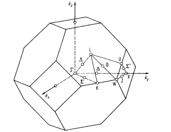
                                                                                                                                                                                                                               Figure 1: Brillouin zone of Silicon (Diamond) structure

 

 

Band structure of Si -

 

• STEP 3: Calculations for bands

 

• Copy Si.scf.in to Si.band.in 

• Edit Si.band.in to perform non-self consistent calculations that will be used to obtain band structure, by setting calculation='bands'.
• Add the parameter in &SYSTEM namelist called nbnd = 8 to specify the number of bands computed. Note that for a 2-atom Si cell, we have 8 electrons and therefore only 4 occupied bands, but we are going to compute some extra (empty) bands.
• Define the K_POINTS card to specify the path along symmetry directions in Brillouin zone. In order to this, you can use the information supplied in the file called k-point-path, which contains a list of k-points along high symmetry directions in the BZ, i.e., L (½, ½, ½) to Gamma (0, 0, 0) to X (0, 0, 1) to W (0, ½, 1) to X (0, 1, 1) to Gamma (0, 0, 0). You can paste that file to Si.band.in after the K_POINTS card. (NOTE: You have change automatic to tpiba which denotes that the k-points are in the units of 2p/a, and also remove the line “6 6 6 1 1 1”).
• Run a 'bands' calculation:
  /usr/local/apps/espresso-5.1/bin/pw.x < Si.band.in > Si.band.out
• What differences do you see between the output file you obtain here, and the output file that you obtained from your scf calculation?

 

 

• STEP 4: Collect band results for plotting

 

• Open bands.in

• Note that you have to use the same prefix in this calculation as was used in scf AND bands calculations.
• The flag filband defines the name of the file in which bands data is to be stored.
• Run:
  /usr/local/apps/espresso-5.1/bin/bands.x < bands.in > bands.out
• Have a look at bands.out and bands.dat and note the minimum and maximum energy eigenvalues at different k-points.

 

 

• STEP 5: Get the data in a format to plot

 

• Open Si.plotband.in

• The first line contains (a) input file (= bands.dat obtained in the earlier step).
• Then (b) Emin and Emax (= -6.00 and 10.00).
• (c) output file in xmgrace format (bands.xmgr)
• (d) output file in ps format (bands.ps)
• (e) Fermi energy (= 6.337 eV)
• (f) deltaE and reference energy (= 1.00 6.337)
• Run the plotting program:
  /usr/local/apps/espresso-5.1/bin/plotband.x < Si.plotband.in > Si.plotband.out
• You can view the plotted band structure written in ps format (bands.ps) using a postscript viewer (e.g., evince).